Binary classification on an email word-count dataset.
This report presents the methodology and visualisation outcomes for binary spam detection using two approaches: (i) logistic regression and (ii) a two-layer neural network with ReLU activation. The dataset comprises 2,736 emails represented by counts of 10 vocabulary words, with a 2,200/536 train–test split. The report focuses on the main concepts, training behaviour, and model comparison, supported by figures that illustrate the learned parameters, predictions, and loss curves. All implementations use only NumPy and Matplotlib, with optimisation via gradient descent (logistic regression) and backpropagation (neural network).
The goal is to learn a predictor that outputs the probability that an email is spam (binary classification). Two models are implemented and compared:
Logistic regression: A linear model that maps a weighted sum of 10 word counts to a probability via the sigmoid function. Parameters are learned by minimising cross-entropy loss with gradient descent over 20,000 steps.
Neural network: A two-layer architecture: 10 inputs → 15 hidden units (ReLU) → 1 output (sigmoid). The network is trained using backpropagation and gradient descent over 100 epochs (one update per training sample per epoch).
This document summarises the most important aspects of both approaches and uses visualisations to illustrate the learned models, their predictions, and their training dynamics. A dedicated Figures section lists all plots with formal captions for reference.
Data: 2,736 emails; each row has 10 word-count features and a binary label (0 = non-spam, 1 = spam).
Vocabulary (order preserved): now, business, click, free, here, money, information, message, research, please.
Split: 2,200 samples for training, 536 for testing. The test set is used only for evaluation to assess generalisation.
Evaluation: Cross-entropy (log) loss on both training and test sets. Lower loss indicates better probabilistic predictions.
The model predicts ( P(t=1 x, ) = (^x) ), where ( (z) = 1/(1 + e^{-z}) ). The parameter vector ( ^{10} ) is learned by minimising the average cross-entropy loss over the training set using gradient descent (learning rate ( = 0.05 ), 20,000 steps).
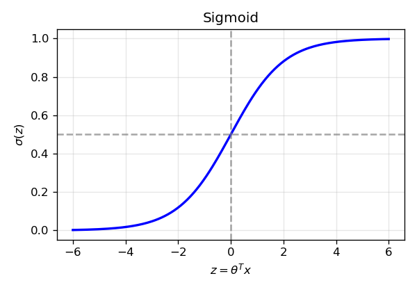
Sigmoid function (Figure 1). The sigmoid maps the linear score ( z = ^x ) to ( (0, 1) ). The plot shows the characteristic S-curve and the decision boundary at ( z = 0 ) (( (0) = 0.5 )).
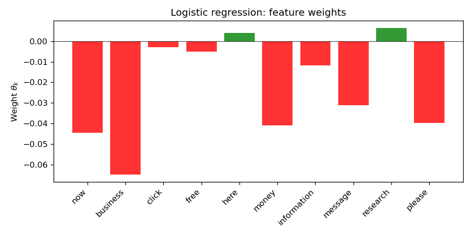
Learned weights (Figure 2). After training, each component of ( ) corresponds to one vocabulary word. Positive weights increase ( P() ); negative weights decrease it. The bar chart reveals which words the model treats as spam-indicative vs non-spam-indicative.
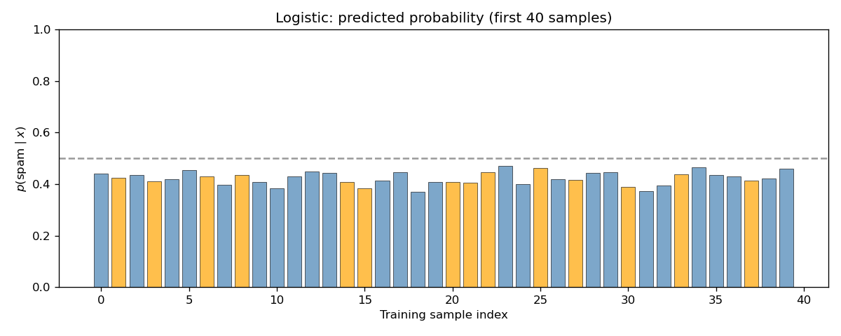
Sample predictions (Figure 3). Predicted ( P( x) ) for the first 40 training samples. Orange bars denote true label spam; blue bars denote true label non-spam. The dashed line at 0.5 is the decision boundary. Good separation corresponds to orange bars above and blue bars below 0.5.
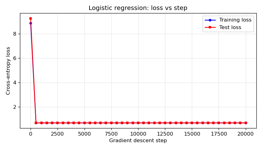
Training dynamics (Figure 4). Training and test cross-entropy loss recorded every 500 gradient steps. Both curves typically decrease and then stabilise. A persistent or growing gap between training and test loss can indicate overfitting.
The network has one hidden layer of 15 units with ReLU activation ( h(a) = (a, 0) ), and an output layer with a single sigmoid unit. The forward pass is:
[ a^{} = W^{} x, h^{} = (a^{}), a^{} = W^{} h^{}, p = (a^{}). ]
Parameters ( W^{} ^{15 } ) and ( W^{} ^{1 } ) are learned by minimising cross-entropy via backpropagation and gradient descent (learning rate 0.05, 100 epochs).
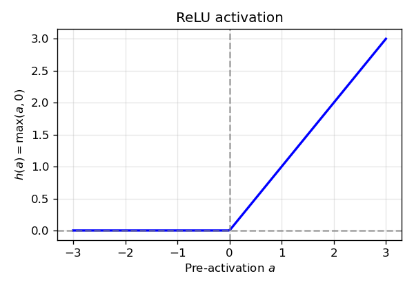
ReLU activation (Figure 5). ReLU zeroes negative pre-activations and preserves positive ones, introducing the non-linearity required for the network to learn non-linear decision boundaries.
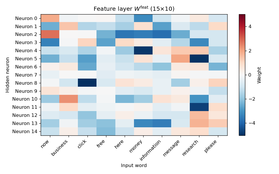
Feature-layer weights (Figure 6). Heatmap of ( W^{} ): rows index the 15 hidden units, columns the 10 input words. Colour indicates weight magnitude and sign. The plot shows how each hidden unit combines word counts.
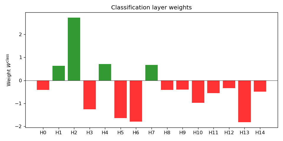
Classification-layer weights (Figure 7). Bar chart of the 15 entries of ( W^{} ). Each bar is the weight from one hidden unit to the output; sign and magnitude show how that unit contributes to ( P() ).
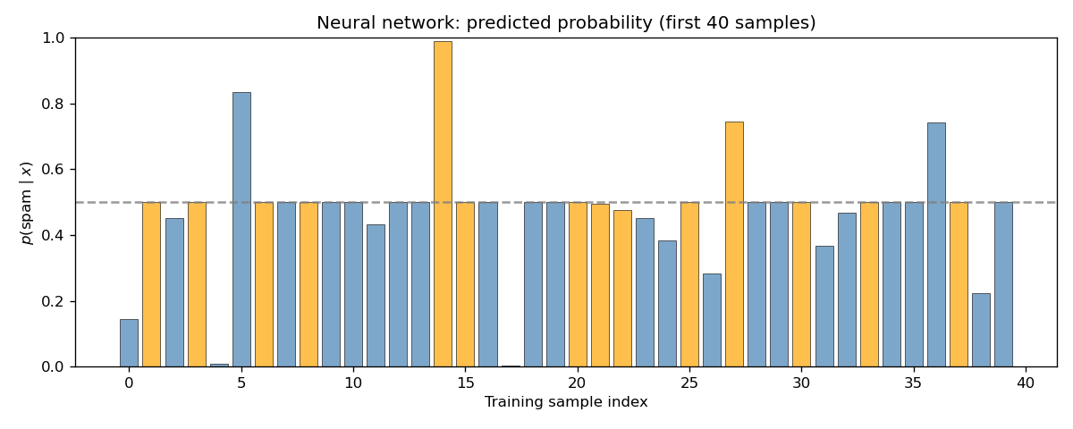
Sample predictions (Figure 8). Same format as Figure 3 but for the neural network. Comparison with Figure 3 shows whether the NN produces more confident or differently distributed predictions.
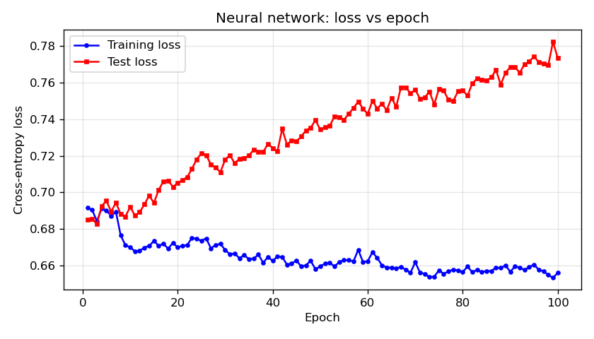
Training dynamics (Figure 9). Training and test loss after each epoch. As in the logistic case, both curves typically decrease then level off; divergence of test loss from training loss can signal overfitting.
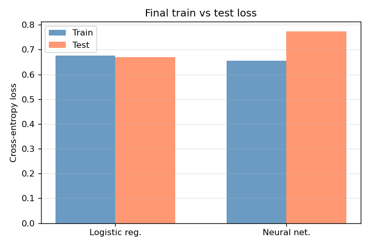
Final losses (Figure 10). Side-by-side comparison of training and test cross-entropy for logistic regression and the neural network. Test loss is the primary indicator of generalisation; the relative performance of the two models can be read directly from this figure.
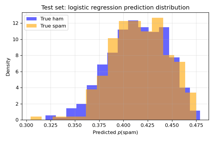
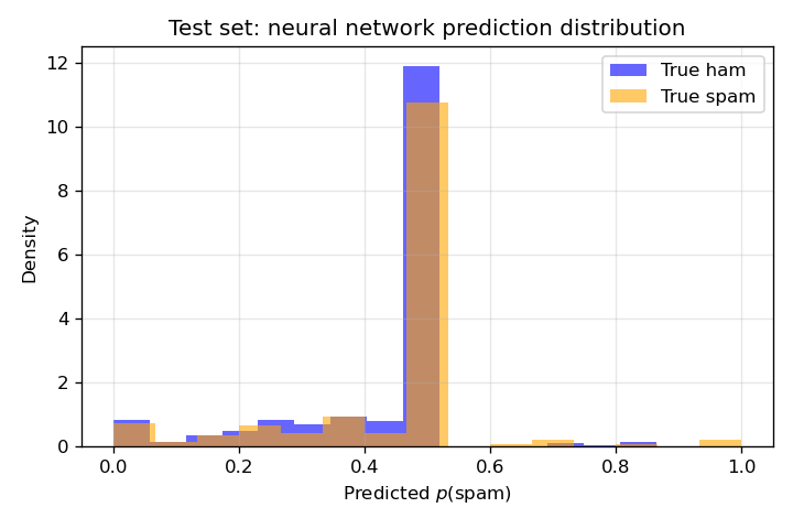
Prediction distributions on the test set (Figures 11 and 12). For each model, predicted ( P() ) on the test set is split by true label: one histogram for true label non-spam (blue), one for true label spam (orange). Well-separated histograms (non-spam near 0, spam near 1) indicate good discrimination; overlap in the middle reflects uncertainty or misclassification. Comparing Figures 11 and 12 shows whether the neural network achieves better separation than logistic regression.
This section lists all figures with formal captions for quick reference.
| No. | File | Caption |
|---|---|---|
| 1 | 01_sigmoid.png | Sigmoid function ( (z) ) mapping the linear score to a probability in ( (0, 1) ). |
| 2 | 02_logistic_theta.png | Learned logistic regression weights ( ) (one per vocabulary word). Green: positive; red: negative. |
| 3 | 03_logistic_sample_predictions.png | Predicted ( P( x) ) for the first 40 training samples (orange = true label spam, blue = true label non-spam). |
| 4 | 04_logistic_loss_vs_step.png | Training and test cross-entropy loss vs gradient descent step (0–20,000). |
| 5 | 05_relu.png | ReLU activation ( h(a) = (a, 0) ) used in the hidden layer. |
| 6 | 06_nn_feature_weights_heatmap.png | Feature-layer weight matrix ( W^{} ) (15×10). Rows: hidden units; columns: input words. |
| 7 | 07_nn_class_weights.png | Classification-layer weights ( W^{} ) (15 values). |
| 8 | 08_nn_sample_predictions.png | Neural network predicted ( P( x) ) for the first 40 training samples. |
| 9 | 09_nn_loss_vs_epoch.png | Training and test cross-entropy loss vs epoch (1–100) for the neural network. |
| 10 | 10_logistic_vs_nn_losses.png | Final training and test loss for logistic regression and neural network. |
| 11 | 11_logistic_pred_distribution.png | Test-set distribution of logistic ( P() ) by true label (non-spam vs spam). |
| 12 | 12_nn_pred_distribution.png | Test-set distribution of neural network ( P() ) by true label (non-spam vs spam). |
This report summarised the two modelling approaches—logistic regression and a two-layer ReLU neural network—for binary spam detection on a word-count dataset. The main visualisations illustrate: (i) the activation functions (sigmoid and ReLU), (ii) the learned parameters (logistic ( ), and ( W^{} ), ( W^{} ) for the NN), (iii) predictions on sample emails, (iv) training and test loss over optimisation steps or epochs, and (v) a direct comparison of both models and their prediction distributions on the test set. Together, these figures support interpretation of model behaviour and of the trade-off between the simpler logistic model and the more flexible neural network.
Figures generated with NumPy and Matplotlib.